Figure 17-1
So far, we have analyzed markets in which price is free to move to the point at which quantity supplied equals quantity demanded. That may not be true if the government imposes a legal maximum or minimum price, or both. If the price control is binding--meaning that the supply/demand equilibrium price is above the maximum or below the minimum permitted--we have a new situation.
You cannot consume something unless someone produces it, so even under price control, quantity consumed and quantity produced must be the same (except in the short run, when you can consume stocks of the good accumulated in the past). If the quantity consumers wish to consume is greater than the quantity producers wish to produce, some mechanism other than price must allocate the limited supply.
In Chapter 2, I briefly discussed one such situation: price control on gasoline. I shall now redo that argument more precisely, using some of what you have learned since.
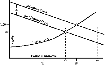
Figure 17-1 shows demand (D) and supply curves for gasoline; they intersect at a price of $1/gallon and a quantity of 20 billion gallons per year. The government imposes price control on gasoline; the maximum price is $0.80/gallon. At that price, producers only want to pump, refine, and sell 17 billion gallons per year, but consumers want to buy 26 billion. Consumers cannot, for very long, use 9 billion gallons per year more than is being produced; gas stations rapidly run out of gasoline. When they do so the cost of gasoline goes up, even though its price does not.
How? One way of making sure you get as much as you want of the limited supply is by getting up early in the morning and arriving at the station shortly after the tank truck leaves. If everyone tries to do that, the result is a long line. Having to wait in line raises the cost of gasoline to the consumer, adding a nonpecuiary cost (a cost in some form other than money--in this case time) to the cost he is already paying in money.
Figure 17-1
The effect of price control on gasoline.
Price control at $0.80/gallon produces a shortage; quantity demanded
is larger than quantity supplied. Lines grow until their cost shifts
demand down to D'. Consumers are paying $0.20/gallon less in money
and $0.30/gallon more in time.
Increased costs due to price control will come in other forms as well. One example is uncertainty--you can never be sure of getting gas when you want it. Every time you take a long trip, you risk being stranded in Podunk. Another additional cost (in time) is making more frequent visits to the gas station in order to be sure your tank is always full. Another may be bribes to the station owner. In at least one case during the gasoline shortage created by the price control of the early seventies, a prominent figure bought his own gas station in order to be sure he and his friends would get gas.
It does not matter, for the present argument, exactly what form the additional cost takes, although it is convenient to think of it, as in the discussion of Chapter 2, in terms of waiting in lines. All we need in order to analyze the effect of price control is the assumption that the additional cost is proportional to the amount of gasoline used (the more you use, the more times you have to wait in line to fill your tank) and is the same for all users. Given those assumptions, we can analyze the effect of price control, using techniques that we developed in Chapter 7 to analyze the effect of taxes.
If I must pay $0.80 in money plus $0.30 in waiting time and other inconveniences for each gallon of gasoline I buy, I will buy the same amount as I would if the price were $1.10/gallon ($0.80 + $0.30). The additional cost is equivalent to a $0.30/gallon tax on consumers; like such a tax, it shifts the demand curve down by $0.30, as shown on Figure 17-1. The time I spend in line is a cost to me but not a benefit to the producers of gasoline; they are still receiving only $0.80/gallon. The effect, on quantity produced and on the welfare of consumers and producers, is the same as if we had simply imposed a $0.30/gallon tax. The only difference is that none of the loss comes back as government revenue.
Thirty cents is not a number picked at random. As you can see on the figure, a $0.30 shift in the demand curve is just enough to make quantity demanded equal quantity supplied at the controlled price. If the cost (of lines and other inconveniences) to the consumers was less than $0.30, quantity demanded would still be more than quantity supplied. The attempts of individuals to compete against each other for the limited supply would drive the cost up further; in the simple example, lines would grow longer.
The startling thing about this analysis is that price control at a below-market price has not only, as one might expect, injured the producers, it has also raised the cost of gasoline to the consumers--by $0.10/gallon. This result does not depend on the details of the diagram. As long as the supply curve slopes up, price plus nonpecuniary cost with price control must be more than price without, although the amount of the increase depends on the relative slopes of the supply and demand curves. In Figure 17-1, the supply curve is twice as steep as the demand curve. Since price determines how much is produced, it is the height of the supply curve at the equilibrium quantity; since cost, pecuniary plus nonpecuniary, determines how much consumers want, it is the height of the demand curve at the equilibrium quantity. As you move left on the figure, the demand curve rises $0.50 for every $1.00 the supply curve falls, so the increase in total cost to the consumers due to price control is half the reduction in price.
The analysis does depend on my assumption that the additional cost is, like a price or a tax, a per-gallon cost--that the increase in the marginal cost of gasoline to the consumer is the same as the increase in the average cost. Usually when we discuss costs to consumers we are talking about prices; the price of a gallon of gasoline is both the marginal cost to you of buying one more gallon of gasoline and the average cost of all the gasoline you buy. That may not always be the case for nonpecuniary costs.
To see why this is important, consider a system of gasoline rationing. The price of gasoline is set at $0.80/gallon, and each year everyone receives ration tickets allowing him to buy 85 percent of what his annual consumption of gasoline was before price control. Anyone who tries to buy more than his ration is shot. Average cost for buying rationed gas is now only $0.80/gallon, but marginal cost beyond the rationed amount is very high--your life for the first pint. People buy until marginal cost equals marginal value--which happens at a quantity equal to what they have ration tickets for, since at that point marginal cost abruptly increases. The situation, for one consumer, is shown in Figure 17-2. The analysis (consumer buys up to that point at which marginal cost equals marginal value) was first done in Chapter 4; the only change is that marginal cost of gasoline to the consumer is no longer independent of quantity and no longer necessarily equal to price.
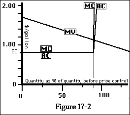
The cost of gasoline under rationing. The
consumer can purchase at the controlled price 85 percent of what he
consumed before price control; additional purchases are illegal.
Once we allow the marginal cost of gasoline to the consumer (which determines how much he buys) to differ from the average cost (which determines how much he pays for it), our proof that price control must injure the consumer is no longer valid. That does not mean that price control plus rationing will necessarily benefit the consumer. He gets gasoline at a lower cost, but he also gets less gasoline. He is better off if the colored area A+C in Figure 17-3 (consumer surplus after price control plus rationing) is greater than the shaded area A+B (consumer surplus without price control) and worse off if it is less.
In more complicated real-world cases, one should also take account of the cost of running and enforcing a rationing scheme and adjusting it to a changing world. During the period of price control and gasoline shortage in the seventies, gasoline was not rationed to individuals but was rationed to regions, on the basis of past consumption; the Department of Energy, in effect, decided how much went where. It has been argued that part of the shortage was caused by the resulting misallocation; the formula used did not take proper account of population movements that were altering the relative demands of different areas of the country.
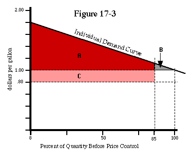
Gains and losses to the consumer due to price
control with rationing. Consumer surplus is A+B before price
control and A+C after; the consumer is better off under price control
if C > B, worse off if C < B.
Gasoline price control--and gasoline shortages--are for the moment only memories, but other forms of price control are still with us. One of the most common, rent control, provides an interesting case for discussing the distinction between allocational and distributional effects.
Economists find it useful to distinguish two sorts of issues, to which they have given the confusingly similar names of "allocation" and "distribution." Allocation is the allocation of goods to people (I get a car with manual transmission, you get a car with automatic transmission, he gets a bicycle: who gets what) or of particular inputs to producing particular outputs (make it this way instead of that way). Distribution is the distribution of real income, including both pecuniary and nonpecuniary benefits (who gets how much). noneconomists tend to think of all issues as distributional: If cars are sold on the market, rich people get them and poor people do not; if we have private schools, rich kids get educated and poor kids don't. Economists tend to be more interested in allocational issues: Consider two people with the same income but different tastes. Let cars and education both be sold. One person buys a car and no education; one buys education and no car.
Economists tend to focus on allocational issues not because distribution is unimportant but because they have less to say about it. Allocational changes typically do--or at least can--benefit (or harm) everyone, so we can evaluate them without worrying about how to balance gains to one person against losses to someone else. Distributional changes are just the opposite. Pure redistribution (I lose a dollar, you gain a dollar, there are no other effects) is neither a gain nor a loss in Marshall's sense. Efficiency is unaffected, and efficiency is the least unsatisfactory criterion we have for judging what is or is not an improvement.
Consider, as a humble example, the common household rule: You made the mess, you clean it up. In any single case, its effects are distributional, since it determines who has to do a particular unpleasant task. Over the long run, however, the distributional effect averages out (unless some members of the household are inherently much messier than others); its main effect is to give people who might make messes an incentive not to do so, and thus produce a more efficient allocation of effort to preventing messes.
One example of the distinction between allocation and distribution and of the difficulty in changing one without affecting the other is rent control. Suppose the city government of Santa Monica decides to impose rent control and sets the maximum rent for each apartment below what its market level would be. The obvious effect is distributional: Landlords are worse off and tenants are better off. The less obvious effect is allocational. At the controlled rent, quantity of apartments demanded is higher than quantity supplied (since at the market rent they were equal). If you are already occupying a rented apartment, you have a good deal; if you are looking for an apartment to rent, you have a problem.
Normally, as families change, they move. A young couple has children and moves from a four-room to a six-room apartment; an older couple moves from a six-room to a four-room apartment after the children leave home. But suppose that, under rent control, the older couple has a six-room apartment for (say) $600/month; controlled four-room apartments rent for $400, and at that price the couple would be happy to move, since the additional rooms are no longer worth $200 to them. But since quantity demanded at the controlled price is larger than quantity supplied, there are no four-room apartments for rent in Santa Monica. Uncontrolled four-room apartments outside of Santa Monica rent for $600. The couple stays in the six-room apartment even though it has two rooms more than they want.
The same problem exists for people who would normally move from a four-room apartment in one part of town to an apartment the same size but in a different location--perhaps because they have changed where they work. If rent control remains in effect for a long time, where people live becomes determined more and more by where they used to live and less and less by where (size and location of apartment) it is now appropriate for them to live. This is an allocational problem: It makes some people worse off without making other people better off.
There is a simple solution. Allow tenants to sublet their apartments--for whatever rent they can get. There will now be two rents for any apartment: the controlled rent ($600 for a six-room apartment in the example we have been discussing) and the rent that a sublessee would pay the original tenant ($800, say) which is what the market rent would have been in the absence of rent control. The cost to an elderly couple of remaining in their six-room apartment is not $600 but $800. If they moved out, they would not only save $600 in rent for themselves, they would also make an additional $200 by continuing to pay rent at $600 and subletting to someone else at $800. Hence they are willing to pay (say) $600 to someone who will sublet a four-room apartment to them, just as (if there were no rent control) they would have been willing to move from an $800 apartment (six rooms) to a $600 apartment (four rooms).
What the combination of rent control plus uncontrolled subletting has done is to permit a free market in apartments while giving the original tenant part ownership of the apartment that he occupied when rent control was imposed. In effect, the tenants of the six-room apartment are quarter owners; if they choose to sublet, they receive $800; three fourths of that goes to the landlord as rent and one fourth they keep. This appears to be a way of producing a distributional effect (which may be "desirable" for political or other reasons) without any undesirable allocational effects.
There are several problems with this. The first is that landlords have almost no incentive to maintain their apartments. In an uncontrolled market, it pays the landlord to make any repairs or improvements that are worth more to the tenant than they cost; he can expect to get the money back in increased rent. Under rent control, all that matters to the landlord is that the apartment be in sufficiently good shape to command the controlled rent. If (as in the example) that is three fourths of the market rent, he can let the apartment deteriorate to three fourths of its previous market value at no cost to himself. The fall in its market rent will all be paid for by his original tenants. If they live in the apartment themselves, they will pay by living in a deteriorated apartment (or maintaining it themselves); if they sublet it to someone else, the deterioration will lower the difference between the rent they pay the owner and the rent they receive from the sublessee.
When rent control has been in effect for a while, apartments start to deteriorate; this results in laws (if they do not already exist) specifying how landlords must maintain apartments. A system of uncontrolled rents in which the landlord was led by his own interest to make those repairs and improvements that were worth making has been replaced by a system of rent control in which uniform standards are set and enforced in order to force landlords to do things that it is no longer in their interest to do voluntarily.
An allocational problem also arises with regard to new construction. Rent control means, in effect, that part of the value of a new apartment building is automatically given to the first set of tenants; they get to rent the apartment from the landlord at the controlled price and to the sublessees at an uncontrolled price. That discourages construction. The obvious solution is to make rent control apply only to buildings that already exist and exempt new construction.
But the same forces that made it politically profitable to impose rent control on existing housing this year (while promising not to control new housing) can be expected to make it profitable, five years hence, to impose rent control on the buildings built during that interval--while promising to leave future construction uncontrolled. Unless the politician not only promises that new housing will not be controlled but also finds some convincing way of committing himself, forcing himself to keep the promise in the future whether or not he still wants to, builders may not believe his promise--and not build. Even if the politician can bind himself, that may merely mean that, five years hence, he will be defeated by another politician running on a platform of controlling the "unfairly" uncontrolled new buildings.
Figure 17-4 shows demand and supply curves for a good whose price is controlled; Pc is the controlled price. To avoid having to shift lines around on the figure, we use a trick introduced in Chapter 7, when we were analyzing the effect of taxes. The supply curve shows quantity produced as a function of price received by the producer; the demand curve shows quantity consumed as a function of cost--price plus nonpecuniary costs--to the consumer.
We begin with price control and no rationing. Lines (or other nonpecuniary costs) grow until they are large enough to reduce quantity demanded to quantity supplied. The nonpecuniary costs are shown on the graph as the difference between price received by the producer and cost paid by the consumer: Cnp on Figure 17-4. The cost of the good to the consumer is the sum of the controlled price and the nonpecuniary cost: Cc=Pc+Cnp. Quantity falls from Qo, the quantity at the market price, to Qc, the quantity supplied by the producers (at a price of Pc) and demanded by consumers (at a price of Cc). The net loss as a result of price control is area B (loss of consumer and producer surplus on goods no longer produced) plus area A (nonpecuniary costs per unit--time waiting in lines and the like--multiplied by the number of units consumed) plus any costs of administering and enforcing the controls.
We now add a rationing system such as that shown in Figure 17-2. Each consumer receives a fixed number of ration tickets, proportional to his previous year's consumption. In order to buy one unit of the good, say one gallon of gasoline, he must pay one ration ticket plus the controlled price of the good.
Under this system, the lines disappear, so the nonpecuniary cost A is eliminated, but new costs are introduced because of the misallocation produced by the rationing system. If, for example, I have just moved from the suburbs to the city, my ration of gas--my previous year's consumption times the ratio of current production to last year's production--is as much as I want at Pc. If the price were any higher, I would not use my full ration. You, on the other hand, have just moved from the city to the suburbs and are desperate for gas. Since your allocation--that same fixed fraction of your previous year's consumption--is far less than you want, you would gladly pay several times the controlled price to get additional gallons. Since I am consuming gas that is worth more to you, we have an inefficient allocation. This time the inefficiency is not only in how much is produced but also in who gets it.
In an ordinary market, producers have an incentive to maintain the quality of their products in order to sell them. Under price control, quantity demanded is greater than quantity supplied; producers find that they can save money by producing a lower quality product and still sell as much as they want at the controlled price. The price control system may be able to prevent some of the more obvious ploys, such as selling three quart gallons at $0.80/gallon, but it is hard to measure and control less obvious dimensions of the product, such as the courtesy and quality of the service provided with the gasoline or the cleanliness of the station's rest rooms. So another cost of price control will be a level of quality below what customers would be willing to pay for on an uncontrolled market--just as one cost of rent control is that landlords no longer have an incentive to maintain their buildings.
Figure 17-4 shows total demand as a function of price; in order to show the effects of inefficient allocation among consumers, we would need to know their individual demand curves and allocations. There is no way to tell from Figure 17-4 how large the resulting loss is; it depends on how accurately the rationing scheme fits the actual demands of the consumers. Net loss due to rationing is now area B plus an unknown additional loss due to misallocation among consumers and inefficiently low quality, plus the costs of running and enforcing the rationing system.
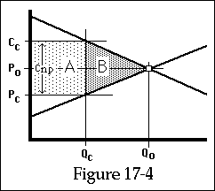
Costs associated with price control. B is a
net loss of surplus due to reduced quantity produced and consumed. A
is the nonpecuniary cost if there is no rationing. It is the total
market value of ration tickets if there is rationing with
transferable tickets.
There is an easy way to eliminate the misallocation: Make the ration tickets marketable. If you want gasoline more than I do, I sell you some of my ration. Under such a system, ration tickets have a market price; at that price, anyone may buy or sell as many as he wishes. Just as for any other good, the price of the ticket will be that price at which quantity supplied equals quantity demanded. The cost of buying gasoline is then the price of gasoline plus the price of a ration ticket. This is obviously true for consumers who use more than their ration and must buy additional tickets: If they want another gallon of gasoline, they must buy both the gasoline and the ticket. It is equally true for consumers who use some of their ration tickets and sell the rest. By consuming a gallon of gasoline from their own ration, they give up the opportunity to sell a ration ticket. The cost to them of consuming the gallon is then its price, Pc, plus the price they could have gotten for the ration ticket they used in buying it.
We know that the quantity of gasoline supplied is Qc. The cost to the consumer at which that quantity is demanded is Cc on Figure 17-4. Since the cost to the consumer is the price of the gasoline plus the price of the ration ticket, it follows that the price of the ration ticket is Cnp--what the nonpecuniary cost would have been without rationing. The price of the ration ticket is serving exactly the same function that the cost of waiting in line served before: reducing the quantity of gasoline that consumers demand to the quantity producers supply. The area A is now equal to the market value of the ration tickets: the number of tickets times the value of one ticket. The net cost is the area B plus costs associated with inefficiently low levels of quality (for gasoline sold at the controlled price) plus any costs of administering and enforcing the rationing.
Aside from administrative costs and effects on quality, the system is precisely equivalent to a tax of Cnp imposed on producers, with the revenue from the tax distributed to consumers in proportion to their previous year's consumption--the same way that the ration tickets are distributed. In both cases, the price received by the producers, the controlled price in the one case or the market price net of tax in the other, is Pc. In both cases, the cost to the consumers of a gallon of gas is Cc. In the one case, consumers get ration tickets with a market value of Cnp dollars each; in the other case, they get an equivalent amount of money.
Why is it that rationing systems usually do not permit individuals to buy and sell ration tickets? Perhaps because that would make the effect of price control plus rationing more obvious--and harder to defend. It is fairly easy to argue that, as a matter of justice, national hardships should be borne by everyone--that if there is "not enough" gasoline, everyone should be allowed to have as much gas as he "needs" and no more--and that the gasoline companies should not be allowed to profit from the shortage. That is a (favorable) description of price control plus a simple rationing system. It is much harder to argue for the peculiar system of taxes and subsidies described in the previous paragraph--which is equivalent to a rationing system after it is improved by making the ration tickets transferable. Yet it is hard to see how one can argue against making ration tickets transferable, since that change benefits everyone: buyers (who get additional tickets for less than they are worth to them) and sellers (who give up tickets for more than they are worth to them).
Can one improve rationing even further in order to eliminate the lost surplus B? Perhaps. The solution is to ration production as well as consumption. Producers must sell a quantity Qc at the controlled price to consumers with ration tickets; any additional production sells at the market price to anyone who wants it (no tickets required). The quantity producers produce depends on their marginal revenue, which is now equal to the market price (since that is the price at which additional units can be sold), so output expands up to Q0, the old uncontrolled output. Having a ration ticket allows you to buy gasoline at the controlled price instead of the market price, so the price of a ticket is the difference between the two prices: P0 - Pc . The system has become a pure transfer of producer surplus to the consumers--very much like the transfer of consumer surplus to the producer under perfect discriminatory pricing. The details of who actually pays are complicated; they depend on how the production ration is divided up among producers and how new producers are treated.
During the oil price control of the 1970s, the U.S. government used such a system of production rationing to control the sale of crude oil to refineries. "Old oil," meaning oil produced by conventional methods from wells that were already producing, was controlled at a low price. "New oil"--oil from new wells, or additional oil produced from old wells in expensive ways, or imported oil--was uncontrolled (the system was actually somewhat more complicated; this is only a rough sketch). Of course, all refiners wanted to buy cheap old oil instead of expensive new oil, so the government rationed the old oil. The rationing rule used was that refiners got allocations of old oil proportional to the total amount of oil they refined. So for each barrel of uncontrolled foreign oil the refiner used, he was entitled to buy a certain amount of cheap, price-controlled domestic oil. These allocations were transferable ration tickets like those discussed above, and were valuable. The government was, in effect, paying refiners to import foreign oil, with the payments coming out of the revenue of the domestic (old) oil producers--a peculiar way of reducing America's dependence on foreign oil.
Back in Chapter 9, we saw that firms in a competitive industry earn no economic profit; if they did, more firms would enter the industry, driving down price and thus profit. The producer surplus of the industry goes not to the firms but to the owners of inputs, such as land or labor. If price control transfers income from the industry to consumers, it must ultimately come not from the firms but from the owners of inputs. In the case of the oil industry, the distinction is in part an artificial one, since oil wells, which are an important input, generally belong to oil companies. What price control of oil expropriated was not the economic profit of the oil companies but part of the quasi-rent that the stockholders of the oil companies were receiving from their past investments in finding and drilling oil wells.
So far, I have considered the distinction between distributional and allocational effects of government decisions in the context of price control; the same distinction is relevant to other issues. Just as in the case of price control, the noneconomist is likely to perceive the issue as purely distributional, the economist as mostly allocational.
One example of this is the issue of who should be liable for injuries caused by defective products. Consider two liability rules: caveat emptor and caveat venditor. Caveat emptor (Latin for "let the buyer beware") means that the seller or producer is not responsible for defects in his product; caveat venditor ("let the seller beware") means that he is.
One's first instinct is to suppose that if the law changes from caveat emptor to caveat venditor, consumers gain (and producers lose) the amount the producers have to pay the consumers to compensate them for defective products. But this conclusion depends on a hidden assumption: that the change in the law will not affect the price at which the goods are sold. That is most unlikely; the new legal rule raises the cost to the producer (when he sells the good, he becomes liable to pay if it is defective) and the value of the good to the consumer. Both the supply curve and the demand curve shift up, so the price must rise.
One's next guess might be that there is no effect at all--the consumers, on average, pay in higher prices just as much as they receive for defective products. This is closer but still not quite right. If the producer is liable for defective products, that gives him an incentive to make the product better. If the consumer is liable, that gives him an incentive to treat the products more gently and to take more precautions to minimize the cost of accidents: wearing safety glasses while using power tools, for instance.
To the extent that the consumer knows how good products are before he buys them, the first incentive is unnecessary--even if the producer is not liable, he will still try to avoid defects in order to make consumers willing to buy his product. Just as in similar cases discussed earlier, the producer will find it in his interest to make any improvements in quality that are worth more to the consumers than they cost him to make, since he can more than cover the additional costs with the increased price the consumers will be willing to pay for the improved product. But to the extent that the cost to consumers of evaluating the products they buy is high enough that they choose to buy in partial ignorance, the incentive provided to the producer by caveat venditor may serve a useful purpose.
This seems to imply that the rule should be caveat emptor where the main danger is from careless use by the consumer or where the consumer can readily inform himself of the quality of the good. It seems to imply that the rule should be caveat venditor where the consumer cannot readily judge quality and the best way to avoid problems is for the producer to produce better goods.
A still better solution is the combination of either caveat emptor or caveat venditor with freedom of contract. Suppose the rule is caveat emptor, and further suppose that consumers would much prefer to buy under a rule of caveat venditor, even at a price that compensated the producers for the cost of that rule. In that case, producers will find that selling their product with a guarantee (at a higher price) is more profitable than selling it without a guarantee. In effect, the producer who offers a guarantee is converting the rule for his product into caveat venditor--he is voluntarily making himself liable for product defects.
Suppose instead that the rule is initially caveat venditor. The consumer can, if he wishes, convert it to caveat emptor in exchange for a lower price--by signing a waiver in which he agrees not to sue. One area where such waivers could make a very large difference is in medical malpractice. Given the high cost of malpractice suits and malpractice insurance, a doctor might offer a much lower price to a patient who signed an agreement not to sue--or even an agreement only to sue in case of gross negligence. Under present law, unfortunately, such a waiver is unenforceable; the patient can sign it before the operation then "change his mind" and sue anyway. That is one example of the general movement of our legal system in recent decades away from freedom of contract, a change that some critics regard as a major cause of the "liability crisis"--the recent sharp increase in the size and frequency of liability suits and the cost of liability insurance.
In discussing gasoline price control, I assumed that all consumers were affected alike by the nonpecuniary costs resulting from a below-market price. A more realistic description would allow for the difference between the cost of waiting in line to a busy professional and the cost to a student who can study while waiting. The nonpecuniary cost must still be high enough to drive quantity demanded down to quantity supplied, but it does so by imposing low costs on some customers (and reducing the quantity they demand only slightly) and high costs on others. The average effect is to injure consumers of gasoline (the increase in nonpecuniary costs is greater than the decrease in price), but there may be many individual exceptions.
Similarly, under rent control, tenants who start with rent-controlled apartments are benefited at the expense of landlords, at least until and unless the apartments are allowed to deteriorate substantially; those who move into the area later, or wish to move from one apartment to another, are injured. There is an obvious distributional transfer from landlords to tenants and a less obvious allocational loss--resulting from misallocation of people to apartments, inefficient levels of construction and maintenance of apartments, and the like.
The same is also true of the change from one liability rule to another. The particular consumer who is injured by an exploding coke bottle may be better off under a rule of caveat venditor--but the consumers who are not injured must pay a higher price because the legal rule raises the producer's cost, the value of the product to the consumer, and hence the supply curve, the demand curve, and the equilibrium price. So they are worse off as a result of caveat venditor. As in the case of gasoline price control, consumers and producers are, on average, worse off as a result of the rule--or of a rule imposing caveat emptor. Both groups would be benefited by freedom of contract.
What these examples suggest is that the effect of market interference is almost the opposite of what one might at first think. One would expect the effect to be mostly distributional, with price control, rent control, or caveat venditor benefiting buyers at the expense of sellers. In fact, it is mostly allocational; the restrictions have as their main effect a less efficient allocation of resources, a smaller pie to be divided up. Such distributional effects as do occur are (except in the rent control case) mostly among consumers and among producers rather than between producers and consumers.
Why is it that rent control, unlike price control of gasoline, has substantial distributional effects? There are two reasons. One is that the supply of housing is, in the short run, very inelastic; landlords do not start tearing down apartment buildings when rents fall by 10 percent. The short-run effect of rent control on the supply of housing is small compared to the effect of gasoline price control on the supply of gasoline.
The other reason is that the tenant who has an apartment when rent control is imposed is like the purchaser of gasoline under a rationing system. He can consume a certain amount of housing and no more (use the apartment he is presently renting) at the controlled price. The additional costs that reduce quantity demanded to quantity supplied affect him only when he wants to move to another apartment. In the short run, rent control is accompanied by a built-in system of rationing: allocate each apartment to the tenant presently living in it. In the very long run, the case of rent control is the same as the case of price control on gasoline--but the short run is long enough so that many individuals benefit for a period of years and sometimes decades, which may explain why it is more popular than most other forms of price control.
In discussing rationing, we found it useful to distinguish between costs that were, like prices, proportional to the amount purchased and costs that were not. In discussing taxes in Chapter 7, I assumed that the tax you paid on something was proportional to the amount of it you bought or sold. That is true of most sales taxes, but it is not true of income taxes in the United States at present.
Under a graduated income tax, your income is divided into brackets, each with a different tax rate. In a progressive system, the higher the bracket, the higher the rate. In a regressive system, the higher the bracket, the lower the rate. While "progressive" sounds as though it means something good and "regressive" something bad, the terms are simply descriptions of two sorts of graduated taxes: one in which rates rise (progress) with income and one in which they fall (regress).
The graduated income tax system of the United States at present is progressive. To simplify the discussion, I will consider a progressive system with a simpler set of brackets and tax rates than we actually have. The first bracket will be from 0 to $10,000/year, the second from $10,000/year to $20,000/year, and the third from $20,000/year up. You pay nothing on income in the first bracket, 40 percent on income in the second, and 80 percent on income in the third.
So if your income is below $10,000/year, you pay no tax; if it is between $10,000/year and $20,000/year, you pay 40 percent of any income above $10,000/ year. If you make $25,000/year, you pay 40 percent of your income in the second bracket (.40 x $10,000/year = $4,000/year) plus 80 percent of your income in the third bracket (.80 x $5,000/year = $4,000/year), for a total tax of $8,000/ year.
An alternative that has been widely discussed is a flat-rate tax. In its purest form, this means that everyone pays a fixed percentage of his income. In considering the effect of shifting from one system to the other, we will discuss first allocational and then distributional effects.
One way of eliminating distributional effects in order to focus on allocational ones is to analyze a situation in which everyone is identical. Suppose, to start with, that everyone has an income of $25,000/year. Under the graduated tax, everyone is paying $8,000/year, which is 32 percent of his income. What would happen if the graduated system were replaced by a flat rate of 32 percent? Would people be better or worse off?
If your answer is "They are paying the same amount in taxes as before, so the change has no effect," you have not yet finished learning to think like an economist. Once people have adjusted to the new tax system, they will be paying more taxes than before--and they will be better off!
Just as the sales taxes analyzed in Chapter 7 affected the amount producers sold and consumers bought, so an income tax affects the amount of their leisure that workers choose to sell. Suppose the wage rate is $10/hour. Under the graduated system, with everyone in the 80 percent bracket, an individual who chooses to sell more leisure--to work more hours--receives only $2 for each extra hour worked; the other $8 goes to the IRS. An individual who sells less leisure--works fewer hours--loses only $2 for each hour less he works. We showed in Chapter 5 that a rational individual chooses to work a number of hours such that the marginal value of his leisure (alias the marginal disvalue of labor) is equal to the wage he receives for working. So each individual works up to the point where the marginal disvalue of one more hour is $2/hour.
Under the new flat-rate tax system, the marginal (and average) tax rate is only 32 percent instead of 80. An individual who works an extra hour at $10/hour receives $6.80 of extra income. After the tax law changes, every worker increases the amount he works (increases the amount of his leisure that he sells, decreases the amount he consumes himself) until the marginal value of his leisure rises from $2/hour to $6.80/hour. The workers are working more hours, receiving more income, paying more in taxes, and are better off.
They are making more because they are working more hours. They are paying more in taxes because 32 percent was the flat rate that would have yielded the same amount as the previous system of rates if incomes had stayed the same. Incomes have risen, so 32 percent of the new income is more than the amount produced by the old system. They are better off not simply because they have more money--that must be balanced against the additional hours they are working--but because each person has chosen an outcome, a bundle of a certain amount of income plus a certain amount of leisure, that he prefers to what he had before.
How do I know that? Under the new system, each individual could choose to work the same number of hours as before and pay the same tax--that, after all, is how the tax rate was calculated. That he does not choose to do so demonstrates that he now has an alternative he prefers. To put the argument more formally, the old optimal bundle is still in his new opportunity set; the fact that it is no longer optimal means that the new opportunity set contains a bundle he prefers to it.
If we now readjust the tax rate (down) so that everyone ends up paying the same tax as under the graduated system ($8,000/year), people are even better off. The flat-rate system now yields government the same revenue while giving every taxpayer an outcome (28 percent, say) that he prefers to the outcome under a flat rate of 32 percent--which he preferred to the old system. The change is not only a Marshall improvement, it is even (under our assumption that everyone is identical) a Pareto improvement.
So far, I have presented the argument in words. Figure 17-5 is a translation of part of it into geometry--specifically, the geometry of budget lines and indifference curves. It shows the alternatives available to an individual who works 250 days a year at $10/hour; each hour/day he works increases his income by $2,500/year. Bp is his budget line under the initial system of progressive taxes. If he works for 4 hours a day (consumes 20 hours/day of leisure) he pays no tax, so he can consume all of the $10,000/year that he earns. On the next $10,000, he pays 40 percent. By working 8 hours/day instead of 4 he increases his income to $20,000 but his consumption to only $16,000; the extra $4000 goes in taxes. His optimum is at point A, where Bp is tangent to indifference curve U1. He chooses to work 10 hours/day, pay $8000 in taxes, and consume $17,000.
Bf shows his situation under a flat-rate tax of 32 percent. If he does not work at all he will have no consumption, so Bf, like Bp, intersects the horizontal axis at 24 hours/day of leisure. If he earns exactly $25,000/year he will pay $8000 in taxes and consume $17,000, just as under the graduated system, so Bf goes through point A.
Since Bf at A has a steeper slope than Bp it must intersect U1 as shown, being above U1 to the left of A and below it to the right. It must therefore be tangent to another and higher indifference curve: U2 at point B. Since U2 is above U1, the taxpayer is better off under the flat rate system. Since the two systems yield the same taxes at point A and B is to the left of A (less leisure, more labor, more income) the taxpayer at B under the flat system is paying more taxes than at A under the progressive system. He is working more hours, paying more taxes, and on a higher indifference curve.
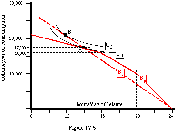
Budget lines for a progressive and a flat rate
income tax. The flat rate is 32 percent, which would bring in the
same amount of money as the progressive tax if the taxpayer worked
the same number of hours under both. In fact, under the flat-rate
tax, the taxpayer works more hours, pays more tax, and is better off.
In proving this result--that a flat-rate tax is unambiguously superior to a progressive tax if all taxpayers are identical--I have skipped over a number of complications. The most important is the effect of the change in the tax law on the wage rate. Unless the demand for labor is perfectly elastic, one effect of an increased supply of labor (everyone is working more hours because of the change in the tax law) will be a fall in the wage rate. A full analysis of the effects of the change would have to take this into account, just as the analysis of the effect of taxes in Chapter 7 included the resulting change in price.
Including that effect would not change the essential result, however; it would simply transform some of the gain from producer surplus (going to the sellers of labor) to consumer surplus (going to the buyers). If everyone is identical, everyone ends up with an equal share of consumer and producer surplus. The analysis would be a little more complicated, but the net effect would still be a gain.
A further complication is the fact that selling leisure is not the only way of getting income; there are other factors of production. The same argument would apply to them as well. An income tax reduces the landowner's incentive to rent out his land, since if he consumes it himself (lives on it) he will get his return in an untaxed form, just as the worker avoids taxes by consuming his leisure instead of selling it. The effect is larger the higher the tax rate. In the same way, an income tax reduces the individual's incentive to save, since part of the interest on his savings will go to the government instead of to him.
One could imagine a variety of other complications as well. So far as I know, none would alter the result. The essential logic of the situation is quite simple. In deciding whether to earn an additional dollar of income, the relevant consideration is how much of that dollar the income earner will be able to keep, so it is the marginal tax rate--the rate paid on each additional dollar of income--that determines how much the taxpayer chooses to earn. Under a progressive system, the marginal rate must be higher than the average rate, hence higher than the flat rate that would yield the same revenue from the same income. From the standpoint of efficiency, the optimal rate is zero, since at a tax rate of zero the individual sells his leisure (or anything else) if and only if its value to the buyer is greater than its value to him--which is the efficient outcome. The flat-rate system has a lower marginal rate, hence is closer to the efficient arrangement, than a progressive system with the same average rate. Since at a lower marginal rate individuals choose to earn more income, the flat rate can actually be below the average of the graduated system and still yield the same tax revenue, making it still more attractive.
The principle here is exactly the same as in the solution to the hero problem of Chapter 1. The hero, as you may remember, is being pursued by 40 bad guys and has only 10 arrows. The solution is to shoot the bad guy in front. Then shoot the bad guy in front. Then shoot the bad guy in front. Then the bad guys start competing to see who can run slowest.
What we have here, just as with the graduated tax (and the ideal rationing system discussed earlier in the chapter) is a discrepancy between an average cost and a marginal cost. On average, the hero can only kill a fourth of his pursuers. But on the margin, the margin of who runs fastest, he can kill all of them--until he runs out of arrows. No one is willing to face a certainty of death just to give the survivors the pleasure of killing the hero. So once he has made it clear what he is doing, they all decline the honor of running in front.
That is also, as you may remember from Chapter 1, how Jarl Sigurd lost the battle of Clontarf: He ran out of men who were willing to carry the banner and accept a certainty of being killed. It is also how you impose a very large penalty for consuming gasoline without actually punishing anyone; if everyone believes he will be shot for exceeding his ration, nobody exceeds it and nobody is ever shot.
As long as we limit ourselves to a world of identical individuals, the case against a progressive tax system is overwhelming. The argument for such a tax system is a distributional one--it is a way of imposing higher tax rates on individuals with higher incomes. In discussing efficiency, I pointed out that most people believe a dollar is worth more to a poor man than to a rich man. If so, a tax system that shifts more of the tax burden onto the rich may produce net benefits--in utility although not in dollars--even if, because of the allocational problems I have just discussed, the rich man is (say) two dollars worse off for each one dollar benefit to the poor man.
The declining marginal utility of income provides one reason why some people might wish to benefit the poor at the expense of the rich, even if there are efficiency costs to doing so. There are others. In Chapter 14, we discussed, but did not resolve, the question of whether the distribution of income produced by the market is in some sense just. For those who decide that it is not, one possible conclusion is that the tax system should be designed to equalize incomes for reasons not of utility but of justice.
Whatever the reason, if one wishes to make the after-tax income distribution more equal than the before-tax distribution, a progressive tax is an obvious--if costly--way to do so. It is not, however, entirely clear whether the tax system that presently exists in the United States has that effect. In analyzing the allocational effects of the two systems, I asserted, and to some degree demonstrated, that complicating the system did not change the essential result. It is less clear whether the same is true of the distributional effects.
It is easier to hide some kinds of income than others. If you are the employee of a large firm and your salary is your entire income, what you report to the IRS is probably very close to what you actually make. If you are self-employed, the opportunities for converting consumption into business expenses for tax purposes--or even concealing income entirely--are much greater. If your income is from capital, you may not be able to conceal it; but you can, at some cost, convert it into capital gains, which were until very recently taxed at a lower rate. Or you can convert your capital into state and municipal securities--which pay a lower interest rate than other investments but are tax exempt.
These complications, and others both legal and economic, imply that the actual tax system redistributes in many different directions. While there is some tendency for richer people to pay more than poorer, thus making the income distribution more equal, there is also a tendency for people with identical incomes to pay very different amounts of tax, thus making the after-tax distribution less equal. Determining what really happens is difficult. The main source of statistics on incomes and taxes is the IRS, and what one is interested in is, in large part, the income that is not reported to the IRS.
Even if the system did, on net, make the income distribution more equal, that would not necessarily mean that the poor would be better off. A more equal distribution would mean a larger share of the pie for the poor; but the allocational costs discussed earlier imply that under a progressive system the pie as a whole is smaller. It is hard to know what the net effect actually is.
One fundamental mistake in popular discussions of this issue and many others is the assumption that what is good for the rich is necessarily bad for the poor, and vice versa. That way of looking at it is an example of the noneconomist's tendency to assume that all issues are distributional. To take a simple counterexample, consider a rich man who is in a 50 percent bracket, earns $200,000/year, and (legally or illegally) conceals most of it--at a cost (to himself) of 45 cents on the dollar. He is behaving rationally--it is worth paying 45 percent to avoid paying 50 percent. If the tax rate falls to 40 percent, he finds it is no longer worth the cost of concealing his income; the rich man is better off, and the IRS collects more money.
The classic example of this phenomenon is due not to Arthur Laffer--who recently popularized it under the name of the "Laffer Curve"--but to Adam Smith. His example was an import duty--a tariff--so high that everything that came in was smuggled. If the duty were lowered to the point where it was no longer worth the cost of smuggling, both consumers and tax collectors would be better off.
1. In my final discussion of price control, I listed a series of alternatives starting with simple price control, going on to price control plus rationing, going on to price control plus rationing plus transferable ration tickets, and ending with all that plus uncontrolled prices for additional output. The examples I used involved oil and gasoline. In the case of rent control, what would correspond to each of those arrangements?
2. Suppose a town has rent control without legal subletting. From time to time an apartment becomes vacant and the landlord decides who he will rent it to. Laws forbidding landlords to accept bribes from prospective tenants are strictly enforced.
How do you think landlords will decide which tenants to rent to? What will the effect be over time on what sort of people rent apartments in that town?
3. The chapter suggests reasons why rent control is more common than most other forms of price control. Give examples of other goods or services that it might be politically profitable to price control for similar reasons. Give examples of goods or services for which price control is very unlikely. Discuss.
4. Regulation Q prohibited banks from paying interest on checking accounts. Banks argued that since this lowered the amount they had to pay to get money, it lowered the amount at which they could lend it out, hence made mortgages less expensive. Discuss.
5. In Chapter 10, I said that Disneyland should charge a per-ride price just high enough to reduce the line at each ride to about zero. Explain why this is true. You will want to combine the analysis of Chapter 10 with the analysis of this chapter. (This is a hard problem.)
6. I demonstrated that in a world of identical individuals, a flat-rate tax was superior to a progressive tax. Is the flat-rate tax the most efficient way of collecting a given amount of revenue in such a world, or is there another alternative that is even better? Discuss.
7. I claimed that the increased income as a result of lowering the marginal tax rate represented a net improvement. Suppose one could somehow impose a negative tax rate: On the margin, for every dollar you earn, the government gives you $0.20. Assuming that the government can get the money in some way that imposes no excess burden, would the resulting increase in the number of hours people worked represent an improvement or a worsening? Explain your answer.
8. Figure 17-5 reproduces only part of the
preceding verbal argument; it does not show the result of reducing
the tax rate to a level that brings in the same amount of tax
($4,000/year) as the progressive system. Draw a new figure showing
the budget line for that rate and the resulting equilibrium point,
along with points A and B and indifference curves U1 and
U2. Draw in additional indifference curves if necessary.