In Chapter 15, I explained the idea of Marshall efficiency and suggested that it could be used as a benchmark for evaluating different economic arrangements. In this chapter we do so, starting with the competitive industry of Chapter 9 and going on to the single-price and discriminating monopolies of Chapter 10. The objective in each case is to prove either that the outcome is efficient or that it is not. To prove that it is efficient, I must show that it cannot be improved by a bureaucrat-god. If it is not efficient, I will prove its inefficiency by showing how a bureaucrat-god could improve it. That may also give us some idea of why it is inefficient and how, even without a bureaucrat-god, the inefficient institutions might be improved.
We assume an industry made up of many identical price-taking firms. The industry sells its output to consumers at a price P; it buys its inputs from the owners of the factors of production: workers, landlords, capitalists. All those involved--firms, consumers, owners--are price takers.
An efficient outcome is, by definition, one that cannot be improved by a bureaucrat-god. We will therefore consider the ways in which a bureaucrat-god might change the outcome produced by the market; if we can show that no possible change is a Marshall improvement, then the original equilibrium must have been efficient.
There are three ways in which the market outcome could be changed. The bureaucrat-god could have the same quantity of the good produced in the same way, while changing its allocation--who gets it. He could produce the same quantity and allocate it to the same people, while changing how it is produced. Finally, he could change the quantity.
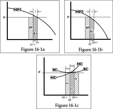
We begin by considering a change in allocation, quantity held constant. Initially, since the good is sold at a price P, everyone who values it at P or higher gets it and everyone to whom it is not worth at least P does not. Figures 16-1a and 16-1b show the marginal value curves of two consumers, Uno and Duo; each is buying the quantity (Q1, Q2) at which his marginal value is equal to P. The total value each of them gets from his consumption is the area under his marginal value curve; his consumer surplus is that total value minus what he pays. To change the allocation we must reduce the quantity consumed by one consumer and increase the quantity consumed by another. Figures 16-1a and 16-1b show the effect of transferring one unit from Uno to Duo.
If we change the allocation without changing any of the associated payments, Uno is worse off by area A1 and Duo is better off by area A2; as you can see from the figure, A1 must be larger than A2. To prove this mathematically, note that since the marginal value curve MV1 is above P to the left of Q1, and the marginal value curve MV2 is below P to the right of Q2, A1 must be greater than a rectangle P high and one unit wide (AP), and A2 must be less than that same rectangle; so A1 > A2. P is a height on the graph ("dollars/unit"), while A1 and A2 are areas (dollars), so we had to convert P into the area P x 1 unit in order to compare it to the areas A1 and A2. You should be able to satisfy yourself that the same relation holds however large the transfer and whatever the shape of the MV curves; the gain to Duo is less than the loss to Uno. Hence the transfer is a Marshall worsening.
Effects of changing the quantity or allocation
of output by one unit. Figures 16-1a and 16-1b show the effects
of transferring one unit of output from Uno (1a) to Duo (1b). Figure
16-1c shows the increased (decreased) cost to a firm of producing one
more (less) unit of output.
The same argument can be made verbally. Before the transfer, everyone is consuming up to the point where MV = P. A transfer from Uno to Duo takes away from Uno units that were worth at least P to him, since at a price P he chose to buy them. It gives to Duo units that are worth less than P to him, since at a price of P he chose not to buy them. Each unit transferred is worth more to the person who loses it (Uno) than to the person who gets it (Duo), so the change is a worsening.
I am measuring value, as usual, by the amount an individual is willing to give up to get something. Some of you may respond that taking steak from a rich man who is willing to pay $4 for it and giving it to a poor man who is willing to pay only $3 is really an improvement, since something worth $3 to the poor man is more important than something worth $4 to the rich man. That is one of the objections to the Marshall criterion discussed in Chapter 15. What it is really saying is that we should maximize total utility rather than total value. But utility cannot be observed and value can. Hence we can describe (and perhaps construct) institutions that maximize total value but not ones that maximize total utility; the former may be regarded as a workable means for approximating the latter.
We have now seen that no reallocation of the existing quantity of output can be a Marshall improvement. The allocation produced by selling the good to all comers at the price at which quantity demanded equals quantity supplied allocates units of the good to those who most value them; any reallocation must transfer from someone who values the units of the good he is losing at more than their price to someone who values the units he is gaining at less. The conclusion holds not only for the quantity of output produced by a competitive industry but for any quantity of output; however much is produced, selling it at the price at which that quantity is demanded is the efficient way to allocate it.
The next question is whether a bureaucrat-god could produce an improvement by changing the way in which the (fixed) quantity of output is produced; after that, we will consider whether he can produce an improvement by changing that quantity.
There are two ways in which the cost to an industry of producing a given quantity of output might be lowered. One is for some firm to produce the same output as before at a lower cost; the other is to change the division of output among firms. But in the initial situation, each firm is already producing its output in the least costly way: Any reduction in cost would increase the firm's profits and so would already have been made. As you may remember from Chapter 9, a firm gets its total cost curve from its production function by finding, for each level of output, the least expensive way of producing it. So there is no way the bureaucrat-god can reduce the cost to the firm of producing a given quantity of output.
What about changing the number of firms: closing down one firm and having each of the others produce a little more or creating a new firm and having each firm produce a little less? Neither of these changes can decrease cost. In equilibrium, as you may remember from Chapter 9, the firms in a price-taking industry are producing at the minimum of their average cost curves--at Q3 on Figure 16-1c. Since the firms are producing at minimum average cost, any change in output per firm must raise average cost, not lower it. Here again, just as in the case of allocation, the result is not limited to the particular price and quantity actually produced. If the demand curve shifted out, increasing price and quantity, the new quantity would again be produced in the least costly way.
We now know that no change in how output is produced or in how it is allocated can be an improvement. In at least these two dimensions, the competitive industry is efficient in the strong sense discussed in Chapter 15; no change that a bureaucrat-god could impose can be an improvement. The one remaining possibility for improvement is a change in the quantity produced.
To see why this also cannot be an improvement, consider Figures 16-1b and 16-1c, which show the marginal value curve of a consumer and the marginal cost curve of a producer. The producer is producing a quantity Q3 for which P = MC = Minimum AC. If he increases output to Q3 + 1, the additional cost will be the area A3. If the additional unit goes to Duo, it will increase his consumption to Q2 + 1; the value to him of the additional consumption is area A2. As you can see from the figure, A3 is greater than AP and A2 is less than AP, so A3 > A2. It follows that the change is a worsening; the gain to the consumer from the additional output is less than the cost of producing it.
The same argument applies if we decrease output instead of increasing it; this time, look at Figures 16-1a and 16-1c. The reduction in output by the firm saves it area A4 < AP, and the loss in consumption to Uno costs him area A1 > AP; again there is a net loss.
What if, instead of increasing output by having one firm produce an additional unit, we increase it by adding one more firm (producing Q3 units) to the industry? The cost per unit of additional output is now only P. But since the value per unit to the consumer of the additional units is less than P, the net result is still a worsening. The same is true if instead of adding a firm and increasing output by Q3, we close down a firm and decrease output by Q3.
The argument can be put verbally as well as graphically. In competitive equilibrium, the price of the good is just equal to the cost of producing a little more or less: P = MC. But since, in competitive equilibrium, consumers buy the good up to the point where its marginal value to them is P, any reduction costs the consumers more than P per unit and any increase benefits them by less. Hence any reduction in output saves the firms less than it costs the consumers, while any increase costs the firms more than it saves the consumers. In competitive equilibrium, consumers are consuming up to the point where each unit is worth exactly its cost of production. Any further increase involves producing units that cost more to produce than they are worth to the consumers; any reduction means failing to produce units that are worth more to the consumers than they cost to produce.
So far, we have only considered changing one variable at a time: allocation, production, or quantity. Could the bureaucrat-god perhaps create a Marshall improvement by changing two or three variables at once? No. We proved that the market allocation rule (sell at the price at which consumers want to buy exactly the amount produced) is the efficient way to allocate any quantity of output and that the way in which a competitive industry produces is the efficient way to produce any quantity of output. So whatever the quantity produced, allocation and production should be done in the way they would be done by a competitive industry. That leaves only one variable--quantity--and we just proved that if output is produced and allocated in that way, the efficient quantity is the quantity a competitive industry chooses to produce.
We are done. We have shown that no change in the outcome produced by an industry of competitive, price-taking firms can be a Marshall improvement. The outcome of a competitive market is efficient.
In presenting the proof that the outcome of a competitive market is efficient, I have deliberately ignored a number of details in order to make it easier for you to see the whole pattern without being distracted by a series of lengthy digressions. I will now go back and fill in the missing points. Two of them are missing pieces of the proof; one is an explanation of something about the proof that you may have found confusing.
Dollar Cost, Value Cost. In demonstrating that the outcome of a competitive market could not be improved, I showed that no change in how the industry produces the output can lower the cost of production. This is not quite the same thing as showing that no change can be a Marshall improvement. A change in cost of production, after all, is merely a change in the number of dollars paid by the firms to the owners of the inputs. What is the connection between showing that a change raises the number of dollars paid ("raises cost") and showing that it is a Marshall worsening ("net loss of value")?
That connection comes from Chapter 5, where we saw that the price of an input (labor in that case) was equal to the cost to the individual of producing it. The marginal disvalue of labor (aka "the marginal value of leisure") was equal to the wage rate. If a producer changes his production process by using an extra hour of labor, the price he must pay for that labor, its cost in dollars, is also the cost to the worker of working the extra hour, its cost in value. By paying the worker his wage, the firm transfers the cost to itself. The worker is neither better nor worse off as a result of working the extra hour (and being paid for it), and the firm is worse off by the amount it has paid. The same analysis applies if the firm uses an hour less of labor--the money saved by the firm is just equal to the value to the worker of the extra leisure he gets. The analysis also applies to the other factors of production, as described in Chapter 14.
What about inputs for which the alternative to consumption by the firm is consumption by individual consumers--apples that can either be turned into applesauce or eaten as apples? Each consumer consumes a quantity of apples for which the marginal value of the last apple is just equal to its price, so if he eats one less apple (because the firm has bought it to make applesauce), the loss of value to him is the same as the dollar cost to the firm. The situation with regard to apples is the same as with regard to labor. If the firm buys an hour of my leisure, I reduce my consumption of leisure by an hour; the cost of doing so is my marginal value of leisure, which in equilibrium equals the price of leisure: my wage. The same is true with apples if we substitute "apples" for "leisure" and "price of apples" for "wage."
This implies that the total cost to the firm of any method of production--any set of inputs--is equal to the sum of the disvalues involved in producing (or not consuming) those inputs. So a change that lowers (dollar) cost also lowers the total value cost of producing the goods--the disvalues of producing the inputs--and a change that increases dollar cost also increases the total disvalues. It follows that a change that raises total cost as measured by firms and changes nothing else must also be a Marshall worsening.
One possibility I have not yet considered is that if the industry uses an additional unit of input, it might get it by bidding it away from some other industry. If the steel industry chooses to use more labor, that may mean not that workers have less leisure but that some workers move from producing autos to producing steel.
What is the cost to the auto industry of losing a worker? It is the worker's marginal revenue product: the increase in output, measured in dollars, from employing him. That, as we saw in Chapter 9, is equal to his wage. His wage is what the steel industry must pay to get him. So the cost in dollars to the firm hiring the input is again the same as the cost in value elsewhere; this time, the loss of value takes the form of lost output in another industry rather than of lost leisure to the worker.
The same argument applies to the other factors of production as well. A firm that increases its use of land by building one-story factories instead of three-story ones does not impose any cost on the land--land does not, like labor, consume its own leisure. It does impose a cost on whoever else is, as a result, not able to use the land. That cost is equal to the rent the firm must pay for the land. A similar analysis holds for a firm that increases its consumption of capital at the expense of other firms.
I have now shown that cost of production as measured by the firms in dollars they spend is the same as the total loss of value from their use of their inputs. Since the competitive industry produces its output at the minimum cost in dollars, it also produces it at the minimum cost in value. So any change in how it produces that quantity of output (everything else held fixed) must be a Marshall worsening.
Shuffling Money. One element in my proof of the efficiency of a competitive equilibrium that may have confused you is the way in which many of the arguments seemed to ignore money payments. I described the cost of an extra hour of labor as its marginal disvalue to the worker, but I then went on to say that the worker was no worse off, since he was paid for his time. I calculated costs and benefits to consumers Uno and Duo by looking at the area under their MV curves rather than by looking at their consumer surplus--the area under the curve and above price. I described the cost to a firm of producing an extra unit as MC, while ignoring the income it got from selling that unit.
All of these features of the proof have the same explanation. A transfer of money from one person to another is neutral in terms of the Marshall criterion, neither a gain nor a worsening. One person gains by a dollar, another loses by a dollar. The only way we can produce improvements or worsenings is by changing what happens with goods: how they are produced, how much of them is produced, who gets them. So when calculating net gains or losses in order to discover whether something is a Marshall improvement or a worsening, we can ignore flows of money.
In discussing the effect of reallocating goods to consumers, for example, I assumed that Uno and Duo continued to pay the same amount of money to the producer as before: The bureaucrat-god simply took one unit of the good from Uno and gave it to Duo. Since there was no transfer of money involved, Uno lost the value of the good to him and Duo gained its value to him.
I could just as easily have assumed that the bureaucrat-god took a unit of the good from Uno and gave it to Duo while at the same time taking P dollars from Duo and giving them to Uno; that would correspond to ordering Uno to buy one fewer good and ordering Duo to buy one more, both at the price P. In that case, Uno would have lost his consumer surplus on one unit (area B1 on Figure 16-2a) while Duo gained his (negative) consumer surplus on one unit (he loses area B2 on Figure 16-2b). He loses because he is buying units for more than they are worth to him, making him worse off than if he did not have to buy them. As you should be able to see from the figures, the net loss if we do it this way, B1 + B2, is the same as A1 - A2 on Figures 16-1a and 16-1b, which was the loss when there was no transfer of money. A1 is AP + B1 and A2 is AP - B2; so AP, the amount of money transferred, cancels, giving us A1 - A2 = B1 + B2.
The same explanation applies to the other cases that may seem puzzling. If a worker is ordered to work another hour and is not paid for it, his cost is equal to his MV of labor. If he is paid for the hour, the cost is transferred to whoever pays him. Net cost is unaffected--we are simply shuffling money.
The same rule of ignoring money payments because they have no effect on what is or is not a Marshall improvement takes care of another problem that may have occurred to you. If a firm decides to increase its consumption of labor, one effect is that a worker works an additional hour. Another effect is that wages rise a little--that is why the worker increases the number of hours he chooses to work. That small increase in wages can be ignored by the firm, since as a price taker it finds the effects of its actions on the prices of the things it buys to be negligible. But for the industry as a whole, or the economy as a whole, that small increase in the wage rate must be multiplied by all of the hours worked by all workers--and the result may not be negligible. Should I not take that into account in calculating the costs and benefits that result from increasing the firm's input of labor by one unit?
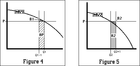
Effect of ordering Uno to buy one unit less and Duo one unit more. AP is the amount spent for one unit; B1 is the consumer surplus loss to Uno and B2 the consumer surplus loss to Duo as a result of the change.
The answer is no. The increase in wages is a transfer between the sellers and the buyers of labor. Each dollar that one person loses, someone else gets. There is no net gain or loss, hence no effect on whether the change is or is not a Marshall improvement. Such "pecuniary externalities" will be discussed in Chapter 18.
One problem with a proof of this sort is that I must present calculus arguments in verbal and graphical form. Strictly speaking, much of the analysis should be put in terms of infinitely small changes: working an extra second rather than an extra hour or consuming one millionth of an apple more or less. Since any large change can be broken up into an infinite number of infinitely small changes, a proof showing that each small change makes things worse also implies that large changes do so. Putting things that way is a good deal harder in a verbal argument than in a mathematical one, but the failure to limit ourselves to infinitesimal changes occasionally introduces errors or confusions into the argument.
It would be possible to give a precise verbal statement of the proof that a competitive equilibrium is efficient, but it would make the proof considerably more difficult than it already is. The proof as given is, I think, sufficiently precise to give you a clear understanding of why the result is true. Readers who feel comfortable with calculus may find it of interest to try to translate the proof into that more precise language.
Competitive Layer Cake. So far, I have described an economy in which there is only a single layer of firms between the ultimate producers and the ultimate consumers. Most real economies are more complicated than that. Many of the outputs of firms--steel ingots, typewriters, railroad transport--are inputs of other firms. While this makes the situation harder to describe, it does not change its essential logic, nor does it invalidate our conclusion that a competitive equilibrium is efficient.
To see why, we will start one layer up from the bottom. Consider an industry that buys its inputs from their original owners (workers, landowners, owners of capital) and produces as output a good used as an input by another firm. The price at which it sells that good equals its marginal cost of production; as we have shown, this is the same as the ultimate cost to those who give up the inputs used in producing it. So when a firm one layer further up uses that good in its production process, the price it must pay for the good is equal to the disvalues involved in producing the good, just as it would be if the good were one of the factors of production instead of something produced by another firm. So our proof of the efficiency of competitive equilibrium applies to the second layer of industry too. We can repeat the argument for as many layers as necessary, thus showing that the whole competitive layer cake is efficient.
A number of other simplifications also went into our argument. One, which has hardly been mentioned so far, is the assumption that each firm produces only one kind of good. Dropping that would make things considerably more complicated and would introduce an interesting set of puzzles involving joint products (things produced together, such as wool and mutton, or two metals refined from the same ore), quality variations among goods, and the like, many of which you may encounter in more advanced texts. It would not change the result.
What about introducing the complications of time and uncertainty that were discussed in Chapters 12 and 13? As I explained there, the effect of time in a certain world can be taken into account by doing all calculations using present values of future flows of revenue, cost, and value. Having done so, we could reproduce the proof we have just gone through and so demonstrate that a competitive equilibrium was efficient in a changing (but perfectly predictable) world.
Efficiency in an uncertain world is a more complicated issue, for two reasons. The first is that, in evaluating outcomes in an uncertain world, we must be careful to specify just what the bureaucrat-god is assumed to know--what sort of "perfect" economy we are using as our benchmark. If the bureaucrat-god knows the future and the real participants in the market do not, he can easily improve on their performance. But in defining the bureaucrat-god, we assumed that he had all of the information any person had, and only that information. That implies that he, like bureaucrats in the real world, has no better a crystal ball than the rest of us. The efficiency proof then holds in an uncertain world as well as in a certain one.
There is another sort of problem introduced by uncertainty that takes us beyond the bounds of this chapter. So far, we have ignored transactions costs, the costs of negotiating contracts, arranging to buy and sell goods, and the like; the only exception was the discussion of bilateral monopoly in Chapter 6. In order to get an efficient outcome in an uncertain world, one must assume that firms can buy and sell a very complicated set of goods--there must be a complete set of markets for conditional contracts. An example of a conditional contract would be my agreement to give you 1,000 gallons of water next year if the price of grain was above $2/bushel and rainfall in Iowa was less than 14 inches.
Such conditional contracts are useful in an uncertain world--you may be an Iowa farmer who only wants the water if both of those conditions hold. But the assumption that there are markets for all of the conditional contracts one can imagine and that on all of those markets transaction costs are negligible is implausible. It is far more implausible than the assumption that in a certain world, where we know what is going to happen next year, there are markets for all goods and that transaction costs on those markets are negligible. Here, as elsewhere, the introduction of transaction costs may invalidate proofs of the efficiency of a competitive equilibrium--or other arrangements. Inefficiencies connected with transaction costs will be discussed at somewhat greater length in Chapter 18.
At the end of Chapter 15, I raised the question of whether efficiency might be an unreasonable standard for judging real-world economies. You are now in a position to see to what degree that is or is not true. I have shown you how a set of institutions--competitive markets--can generate an efficient outcome, in the full sense in which the term is used in Chapter 15--an outcome that cannot be improved by a bureaucrat-god. I have also, I hope, given you some feeling for why that is only an approximation, although not a wildly unreasonable one, of a real economy.
Throughout the argument, I have assumed that everyone concerned--firms, owners of the factors of production, and consumers--is a price taker. If even a single participant in the market is not, then somewhere in the chain of argument a link fails and we can no longer prove efficiency.
As you may suspect from the amount of space I have spent on this discussion and the number of different things from different chapters that have fed into it, the efficiency of a competitive market is an important result. Insofar as one is interested in using economics to improve the well-being of mankind, it is probably the most important single result of economic theory. While we cannot expect any real-world economy to fit the requirements of the proof precisely, many economies, or at least many parts of many economies, come close enough to make us suspect that they are very close to being efficient--closer than under any alternative institutions. Where the assumptions necessary to prove efficiency break down, as in the case of the price-searching firms discussed in Chapter 10, understanding why the failure of the assumption leads to a failure of the proof is the obvious starting point for anyone who wishes to figure out how the situation could be improved.
So far, we have been analyzing the efficiency of the outcome of a competitive industry, an industry in which all participants are price takers. We will now consider the case of a monopolistic industry. Just as in Chapter 10, we will start with a single-price monopoly and then go on to more complicated cases.
One of the difficulties in teaching (and learning) economics is that many students start out believing they already know it. The subject is the world we all live in, and many of the words are ones whose meaning everyone already knows. It is easy to forget that a term such as "efficient" or "competitive," when used in economics, is a technical term with a meaning quite different from the same term used in ordinary conversation.
One of my favorite examples of this problem is the sentence "Monopoly is inefficient." The natural response of a student hearing or reading that sentence is, "Of course; I already knew that. Monopolists are rich and lazy; they have no competitors to put pressure on them, so they run their firms badly."
As you will see shortly, rich and lazy monopolists running their firms badly have nothing at all to do with what an economist means when he says that monopoly is inefficient. Indeed, in the sense in which "efficient" is used in ordinary conversation, economic theory suggests that monopolies should be just as efficient as competitive firms. It is only in the very different sense of "efficient" discussed in the previous chapter that we have reasons to expect at least some kinds of monopolies to be inefficient--not because the monopolist runs his firm badly but because he runs it well.
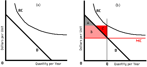
Consider the firm whose marginal cost, marginal revenue, and average cost are shown on Figure 16-3, along with the demand curve for its product. It costs the firm $1,000 to produce any widgets at all and $10/widget for each additional widget it produces, so its fixed cost is $1,000/year and its marginal cost is $10/widget. Since the firm has positive fixed cost and constant marginal cost, average cost is lower the more the firm produces; the more widgets it is divided among, the lower the fixed cost per widget. The result is a natural monopoly; the larger the firm, the lower its average cost. As we saw in Chapter 10, the firm maximizes its profit by producing a quantity for which marginal revenue equals marginal cost.
Is this efficient? Our proof of the efficiency of a competitive industry involved three parts: efficient allocation of output, efficient production of output, and efficient quantity of output. So far as allocation is concerned, the proof applies to the single-price monopoly as well; it, like a competitive industry, sells its goods at the price for which quantity demanded equals quantity produced. Any reallocation of the existing quantity of output must transfer a good from someone to whom it is worth at least its price to someone to whom it is not, so it must be a Marshall worsening.
The proof also holds with regard to production efficiency. If the firm could produce the same quantity of output at a lower cost it would, since a reduction in cost would increase profits. Nor can the cost of production be lowered by a change in the number of firms. Since the firm is a natural monopoly, any increase in the number of firms must raise average cost. So the monopoly industry is efficient both in how it allocates its output and in how it produces it.
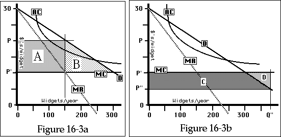
The profit-maximizing price (P) and the
efficient price (P') for a single-price monopoly. Lowering the
price from P to P' (Figure 16-3a) lowers the monopoly's profit by A
but increases consumer surplus by A + B for a net gain of B. A
further reduction to P" (Figure 16-3b) would cost the monopoly C + D
and benefit consumers by C, for a net loss of D.
What about the quantity it chooses to produce? The firm charges a price P at which MC = MR, since that maximizes its profit. If it lowered its price to P' = MC = $10/widget, its profit on the 150 widgets per year that it had been selling for a price P would decline by the area A, since it would be selling those widgets for a price of only P'. At a price of P', it would also be producing and selling an additional 150 widgets per year, for a total of 300. It would neither make nor lose money on those additional widgets, since they would each cost $10 to produce (MC) and would each be sold for $10.
The drop in price would benefit consumers by area A plus area B--the increase in their surplus. Area A is the savings on the widgets they would have bought at the old price; area B is the consumer surplus on the additional widgets. Since the change benefits the consumers by more than it costs the producer, the decrease in price from P to P' is, on net, an improvement.
Would lowering the price even further improve things even more? No. A further price change to P" = $5/widget, as shown in Figure 16-3, would cost the producer an amount equal to the area of the entire colored rectangle C + D = Q" x (P' - P") and benefit consumers by the lightly colored area C; there would be a net loss equal to the area D. You should be able to convince yourself that at any price above or below P' = MC, net benefit is less than at P'. The efficient arrangement is for the monopoly to charge a price equal to marginal cost.
The same argument can be made verbally without using the figure. As long as price is above marginal cost, there are people who value an additional widget at more than it would cost to produce it; producing that additional widget and giving (or selling) it to such a person produces a net benefit. If the price were below marginal cost, some people would be consuming widgets that were worth less to them than the cost of production; reducing the production and the consumption of such a person by one widget would produce a net benefit. So we get an efficient outcome only with price equal to marginal cost. This is the same rule that defines the efficient price for a competitive industry.
But while price equal to marginal cost maximizes net benefit, it does not maximize the monopoly's profit; if the monopoly shown on Figure 16-3 sold at $10/widget (MC), it would just cover its variable cost and lose $1,000/year of fixed cost. It prefers to charge price P, corresponding to a quantity for which marginal cost equals marginal revenue, instead of P' = MC. So a single-price monopoly will charge an inefficiently high price--not because the monopolist does not know how to maximize his profit but because he does.
A competitive firm, on the other hand, charges a price equal to marginal cost; the same argument shows that that is the efficient arrangement. It would seem to follow that there is an efficiency gain to breaking up a single monopoly firm into many small firms.
A glance at AC on Figure 16-3 should convince you that that is wrong; if the firm is broken up into ten smaller firms, average cost will be much higher and the price will go up instead of down. Not only that, but the situation will be unstable. Since average cost falls as output increases, one of the firms will expand, driving (or buying) out the others. We will then be back where we started, with a single monopoly firm.
What the demonstration does imply is that if the cost curves are consistent with competition, as in Figures 16-4a and 16-4b, a competitive industry results in a greater net benefit than a monopoly. This is an argument not against natural monopolies but against government-enforced monopolies (or cartels) in naturally competitive industries, such as trucking or agriculture. In Figure 16-4a, the average cost for a large firm (producing Q2) and a group of small firms (producing Q1 each) are the same, so the loss due to a government-enforced monopoly is the loss of the area B, the consumer surplus on the goods that would be produced if the industry were competitive but are not produced when it is a monopoly. In Figure 16-4b, the large firm has larger costs than the small, as we would expect in a naturally competitive industry, so there is the additional loss of the area B', equal to the difference in average cost between five small firms and one large one times the monopoly output.
The same analysis also demonstrates the undesirability of artificial monopoly and so provides an argument in favor of government antitrust measures designed to discourage it. I argued in the optional section of Chapter 10 that attempts to establish artificial monopolies, monopolies formed and maintained in industries where a monopoly firm has no advantage in production costs over a smaller firm, are unlikely to succeed. If that conclusion is correct, there is no need for antitrust laws to prevent them; if it is wrong, the argument for the inefficiency of monopoly is an argument for antitrust.
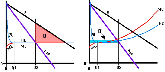
Efficiency gains from breaking up an
"unnatural" monopoly. Figure 16-4a shows the case where a large
firm has the same average cost as a small firm; B is the gain from
increased output when the industry becomes competitive. Figure 16-4b
shows the case where cost is larger for a larger firm; breaking up
the monopoly then also reduces total production cost by B'.
What about the hard case: the natural monopoly illustrated in Figure 16-3? The government could pass a law requiring the firm to sell at a price equal to marginal cost--but the firm would respond by going out of business, since at that price it is losing money.
One solution is for the government either to regulate the monopoly or to run it, charging a price equal to marginal cost and making up any loss out of tax revenues. This leads to a number of additional problems.
Regulation and the Second Efficiency Condition. In the previous section, I demonstrated one efficiency condition for a monopoly: Price equals marginal cost. That condition determines how much a monopoly should produce, since price (and the demand curve) determines quantity. There is a second efficiency condition, which determines whether the monopoly should produce anything at all. Figure 16-5a shows cost curves and a demand curve for a firm whose fixed cost is so great that average cost is always above the demand curve. Whatever quantity of output it chooses, its average cost of production will be higher than the price at which it can sell that quantity. Such a firm would never come into existence; if it did, it would go out of business as soon as its owners recognized the situation.
Should such a firm come into existence? Will net benefit be higher if it exists? That depends. If it produces a quantity Q at price P = MC, as shown on Figure 16-5b, the firm will lose its fixed cost and its customers will gain their consumer surplus. If the consumer surplus is larger than the fixed cost, there is a net benefit (although the firm still loses money); if the consumer surplus is less than the fixed cost, there is a net loss. Our first efficiency condition was "Price equals marginal cost"; our second is "Produce only if, at the quantity for which price equals marginal cost, consumer surplus plus profit is positive" or, in other words, consumer surplus is larger than the loss to the firm, if any.
Looking at a graph such as Figure 16-5b, how can one tell whether the loss to the firm is more or less than the gain to its customers? We know that if the firm exists, it should produce quantity Q. If it does, consumer surplus will be the triangle A+B. On average, the firm makes P - AC on each of Q units; since P is less than AC, it is losing the rectangle B+C. If A+B is larger than B+C, or in other words if A is larger than C, the firm is producing a net benefit. If C is larger than A, it produces a net loss.
A private, profit-maximizing monopoly will only produce when profit is positive (or zero), in which case profit plus consumer surplus must be positive. So it will never produce when, according to the second efficiency condition, it should not. It may, however, fail to produce when it should--if profit is negative but the loss to the firm is less than the gain to its customers. In addition, as pointed out above, such a firm will not meet the first efficiency condition, since it will set marginal revenue equal to marginal cost instead of price equal to marginal cost.
Can a government-owned or government-regulated monopoly do better? It is not obvious that it can. There are two sorts of problems that it faces. First, there are problems associated with getting the regulatory agency to do what it "should" do. There is no obvious reason to expect the commissioners of a regulatory agency, or the official in charge of a government monopoly, to have any more interest in maximizing net benefit than the owner of a private monopoly. Regulators may well find it in their interest to regulate a monopoly in some way other than that recommended by economists. They might choose to allow the monopoly to make large profits in exchange for political contributions to the incumbent administration or future high-paying jobs for the regulators, or they might force the monopoly to provide service at a price below marginal cost in order to buy popularity with consumer-voters at the expense of the monopoly firm's stockholders. A regulator, or an official running a government monopoly such as the U.S. Post Office, is presumably trying to maximize some combination of private benefit to himself and political benefit to the administration of which he is a part; it is not obvious that he does either by maximizing net benefit to producers and consumers.
A natural monopoly that cannot cover its
costs. Since for any quantity of output, AC is above the price
that quantity sells for, a single-price monopoly cannot cover its
costs. If such a monopoly operates and sells at P = MC, A+B is the
gain to its customers and B+C the loss to the monopoly firm.
Government regulation or ownership of monopolies is what economics textbooks have traditionally offered as the cure for the efficiency problems of private monopoly. What is wrong with this traditional analysis is that it treats the owners and managers of a private monopoly as part of the economic system, acting to achieve their own objectives, but treats government officials as if they were benevolent bureaucrat-gods, standing outside the system. There seems no good reason for such an asymmetrical treatment of the two alternatives. In Chapter 19, we will see the results of including government within our analysis, applying the same assumptions to the participants in the political market as to the participants in the ordinary market.
Suppose, however, that the regulators do have the best of intentions; their only objective is to maximize net benefits by forcing the firm to follow the prescription of the two efficiency conditions: Charge marginal cost, provided that at that price net benefit is positive. They will find it difficult to do so.
In order to keep the regulated firm of Figure 16-5 in business, someone, presumably the government, has to make up the firm's losses: the difference between what it costs the firm to produce its output and what it is allowed to sell it for. If the government simply provides a subsidy equal to the difference between the regulated firm's revenue and its costs, the management of the firm has no incentive to keep down costs--especially the cost of things that can be used to make the life of management easier. If, instead, the regulatory agency estimates what marginal cost and average cost ought to be and offers the firm a fixed subsidy to cover the difference (while ordering it to sell at marginal cost), the firm has an incentive to misrepresent its cost function so as to make average cost appear as high as possible. The regulators must come very close to running the firm themselves if they are to guarantee both that price equals marginal cost and that the total cost for producing whatever level of output can be sold at that price is as low as possible.
Suppose we assume these problems away too; we assume not only that the regulatory commission is trying to maximize net benefit but also that it knows the firm's cost curves. Even under these rather implausible assumptions, there is still a problem with the conventional regulatory solution to natural monopoly.
The problem is the second efficiency condition. The combination of marginal cost pricing plus a subsidy to cover the resulting loss will permit a monopoly to stay in business even if it does not meet the second efficiency condition--even if its costs are larger than the value to its customers of what it produces. In order for the regulatory agency to subsidize only those monopolies that should stay in business, it must know not only the cost curves of the firm but also the demand curve for its output, so that it can calculate what consumer surplus will be if the firm sells at marginal cost. If the consumer surplus is less than the required subsidy, the firm should be allowed to go out of business. But all the agency can observe directly is one point on the demand curve: quantity demanded at a price equal to marginal cost. That point gives very little information about consumer surplus; through the same point, one can draw two demand curves (D1 and D2 on Figure 16-6), one of which yields almost no consumer surplus at a price equal to marginal cost and one of which, at the same price, yields a very large consumer surplus.
Can the regulatory agency determine the demand curve by asking the monopoly's potential customers how much they would buy at each price? Not if the customers are rational. However much the customers say they would pay, if the monopoly produces they will only be charged marginal cost. It is in their interest to have the monopoly produce, since the customers receive all the benefit and pay only a small part of the taxes for the subsidy; so it is also in their interest to lie about how much it is worth to them, exaggerating the figure in order to induce the agency to subsidize the monopoly.
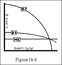
Two different demand curves that result in the
same quantity demanded at P = MC.
It seems that even a benevolent and well-informed regulatory agency faces a nearly insuperable problem in deciding which monopolies should be subsidized in order to keep them in business. An unregulated single-price monopoly may sometimes face a very similar problem. Consider the case of an unregulated railroad deciding whether to build a new rail line, and contrast it to the case of a regulatory agency deciding whether to subsidize the construction of a new rail line. The regulatory agency wants to maximize total value; the unregulated monopoly wants to maximize its profit. Each, in order to achieve its goal, must first estimate demand and then decide whether the rail line should be built.
There is one important difference between the two cases. The unregulated monopoly discovers, after the line is built, whether its decision was correct; there either is or is not some price at which the monopoly can make a profit on the new line, and it soon learns which. Since it can recognize success and failure, it can continually improve whatever techniques it uses to estimate demand; crudely speaking, if it builds a line and loses money, it can fire the market researchers who told it to build the line. The regulatory commission has no comparable test; even after the line is built, the commission never learns whether the line was worth building, since all the commission observes is quantity demanded at price equal to marginal cost.
Nationalized Monopoly. It is sometimes suggested that the government, instead of regulating natural monopolies, should nationalize them and run them itself "for the public good." This solves one of the problems of regulated monopoly. The regulatory agency no longer has to duplicate the work of management in order to get the information necessary to regulate; now the agency is the management of the firm. It does not solve the incentive problem; it is by no means obvious that the interests of the managers of a nationalized firm, or of the politicians who appoint them, are the same as the interests of the population as a whole. Nor does it solve the problem of satisfying the second efficiency condition.
There is at least one important respect in which both regulation and nationalization may be worse than unregulated single-price monopoly. So far in this chapter, I have described natural monopoly as if it were an all-or-nothing matter. In fact, there are many intermediate points between perfect competition and natural monopoly, and the location of a particular industry along that continuum may change. In the case of an unregulated natural monopoly, if conditions change so that it becomes possible for smaller firms to enter the industry successfully, they will do so; the monopoly will gradually break down. If the industry is regulated or nationalized, the regulatory agency or the nationalized industry may use the force of law to control or prevent new competitors, thus converting the industry into a government-enforced monopoly. An example is the regulation of transportation by the Interstate Commerce Commission. In the absence of regulation, the transportation industry would have become competitive when trucking developed as a major competitor to rail transport, since large trucking firms have no important advantage in production cost over small ones. The ICC regulated--and to a considerable degree cartelized--the trucking industry in order to protect its original regulatees, the railroads.
So far, we have only considered single-price monopolies; we will now shift to the opposite extreme and consider a perfectly discriminating monopoly. Since it can sell at different prices to different customers, or sell to a single customer at a range of prices, it always pays the monopoly to produce and sell to any customer who is willing to pay, for one more unit, more than its marginal cost. So it sells the same amount, to the same people, as it would if it were selling at marginal cost.
The difference is that what would be consumer surplus for the single-price monopoly selling at marginal cost becomes revenue for the perfectly discriminating monopoly. Since the monopoly is collecting the sum of producer and consumer surplus, it is in the monopoly's interest to maximize that sum; so a perfectly discriminating monopoly satisfies both the first and second efficiency conditions! The information needed to satisfy the second efficiency condition--the shape of the demand curve--is part of the information that a firm needs in order to be a perfectly discriminating monopoly. And unlike the regulatory commission, the firm, having made an estimate of the shape of the demand curve, tests it by its pricing scheme. If, for example, the firm uses two-part pricing (per widget plus entry fee), an overestimate of consumer surplus will result in too high an entry fee and no customers.
This result holds only for a perfectly discriminating monopoly. Monopoly with imperfect price discrimination not only fails to produce an efficient outcome, it may produce a worse outcome than single-price monopoly. Since it charges different prices to different customers, it, unlike a single-price monopoly, allocates its output inefficiently. If two customers paying different prices each buy up to the point where price equals marginal value, the high-price customer will value his marginal unit more than the low-price customer, so a transfer from low-price to high-price customer would produce a net benefit. This inefficiency in allocation may or may not be balanced by an increase in output, relative to what would be produced without price discrimination, depending on the details of the situation.
The arguments I have given so far suggest that a perfectly discriminating monopoly, insofar as it is feasible, is the ideal solution to the problem of natural monopoly. It is ideal in that it maximizes total value, although it does so in a way that gives all the net value resulting from the monopoly's activities to the monopoly instead of leaving some of it with the customers. If we look at this situation from a point of view sufficiently broad to give the same weight to the interests of the stockholders of the monopoly firm as to those of its customers, the only defects to this solution seem to be the considerable difficulties in actually running a perfectly discriminating monopoly.
There is another and more profound difficulty with this solution. A perfectly discriminating monopoly, or even an ordinary single-price monopoly, receives profits above and beyond the normal return on capital. Firms therefore compete to become monopolies. If we consider such competition as itself an ordinary profit-maximizing economic activity, we expect that a firm will be willing to spend, in the attempt to become the monopoly, anything up to the full value of the expected profits. Insofar as this expenditure does not produce anything for anyone (aside from getting that firm, instead of another firm, the monopoly), it is sheer waste. If the firm consumes the full value of the monopoly in the process of getting it, and if, as in the case of perfectly discriminating monopoly, that value is the entire value to all concerned from the existence of the industry (consumer plus producer surplus), then the private perfectly discriminating monopoly, rather than being the best possible solution to the problem of natural monopoly, is the worst. The industry generates no net value to anyone.
This point can be clarified by an example. Suppose there is a certain valley into which a rail line could be built. Further suppose that whoever builds the rail line first will have a monopoly; it will never pay to build a second rail line into the valley. To simplify the discussion, we assume that the interest rate is zero, so we can ignore complications associated with discounting receipts and expenditures to a common date. Assume that if the rail line is built in 1900, the total profit that the railroad will eventually collect will be $20 million. If the railroad is built before 1900, it will lose a million dollars a year until 1900, because until then, not enough people will live in the valley for their business to support the cost of maintaining the rail line. Lastly, suppose that all of these facts are widely known in 1870.
I, knowing these facts, propose to build the railroad in 1900. I am forestalled by someone who plans to build in 1899; $19 million is better than nothing, which is what he will get if he waits for me to build first. He is forestalled by someone willing to build still earlier. The railroad is built in 1880--and the builder receives nothing above the normal return on his capital for building it.
This phenomenon--the dissipation of above-market returns in the process of competing to get them--has recently become known as rent seeking. It is a new and somewhat complicated subject; the results are not always as perverse as in this example. One can, for instance, add the additional assumption that there exists a strip of land that controls the only potential rail access to the valley. In this case the $20 million profit, instead of being dissipated by building the railroad early, goes to the person who owns that strip of land and auctions it off to the highest bidder--who then waits until 1900 to build his railroad, making perfect discriminatory pricing again the perfect solution to the problem of natural monopoly.
The analysis of rent seeking suggests that, at least under some circumstances, monopoly profit is not a transfer to the firm from its customers but a net loss. The higher the monopoly profit, the more resources the firm will burn up (by, in our example, premature construction of the railroad) in the process of getting it. If so, perhaps the best solution to the problem posed by monopoly is not regulation but taxation--taxation not of output but of profit.
Suppose the government imposes a 50 percent tax on the economic profit of a monopoly. Since the firm still gets 50 cents out of every dollar of profit, it is still in its interest to make profit as large as possible; so it behaves exactly as it would without the tax--produces the same quantity at the same price. Since the tax has no effect on the behavior of the firm, there is no excess burden. If the firm would otherwise have spent the present value of its anticipated monopoly profit in gaining the monopoly, then the knowledge that it will get only half as much will cut in half the amount it spends in rent-seeking behavior--the railroad, in our example, will not be built until 1890. In this case, the tax not only has no excess burden, it has no burden at all! What the government collects would otherwise have been wasted in premature construction.
The most obvious difficulty with this proposal is that in order to tax something you must first be able to identify it, and monopoly profit is easier to identify on a figure in a textbook than in the real world. A firm that appears to be making large profits may be a successful monopoly, but it may also be a firm in a competitive industry that gambled on a new product or a more efficient method of production and won. If profits above the market rate are automatically identified as a sign of monopoly and taxed accordingly, one result will be to reduce the incentive for such innovations.
There is an elegant solution to this problem. Suppose we know in 1900 that, starting in 1920, the American aluminum industry will be a natural monopoly. Let the government auction off the monopoly--the right to produce aluminum after 1920--to the highest bidder. Aspiring monopolists should be willing to bid up to the full present value of the future monopoly profits, so the government will have collected a 100 percent tax on monopoly profits, as estimated by the (prospective) monopolist.
This solution again has a problem--it depends on our being able to identify natural monopolies, and to do it even before they exist. If we guess wrong, we have just auctioned off a monopoly of a potentially competitive industry, and thus produced a governmental monopoly with its associated costs.
Even if we could identify natural monopolies correctly, it is not clear we would. The arguments of the last few paragraphs could, after all, provide elegant camouflage for a government that wanted to create monopolies, either as a source of revenue or in exchange for political support by favored firms and industries. It is worth remembering that the term "monopoly" originated in just this context--to describe otherwise competitive industries, such as the sale of salt, where one producer had bought from the government the right to exclude all others.
The great mistake in most discussions of the problem of natural monopoly is the assumption that the problem is monopoly. The problem is a particular kind of production function: one for which minimum average cost occurs at a quantity not much less than the total amount of the good produced and sold. A single-price private unregulated monopoly is one (imperfect) solution to the problem posed by such a cost curve. It is imperfect because although it is efficient in the sense of producing a given quantity of output at the lowest possible cost, it is inefficient in both the quantity it produces (too low) and its decision of whether to produce at all (sometimes it will not when it should). Regulated private monopoly is another imperfect solution, one that may do better than unregulated private monopoly with regard to quantity but worse with regard to least-cost production, and that is less likely to disappear when and if the problem disappears. Government-run monopoly is yet another imperfect solution, with many of the same problems. Perfectly discriminating monopoly, to the extent it is possible, is an elegant solution that avoids the defects of the other alternatives only to introduce a potentially worse defect in the form of rent seeking.
In several places in the text, you have been told that a single-price monopoly is inefficient; since it sells at a price above marginal cost, there will be some customers willing to pay more than the cost of production who do not get the good. If the monopoly lowered its price to MC and increased production accordingly, there would be a transfer from it to its present customers plus a net gain on the increased production.
This is true for the monopoly resulting from a patent or copyright, just as for other monopolies. The owner of a patent or copyright charges a licensing fee to the producer for each unit produced; this raises the price above the true marginal cost, since part of the cost the producer pays on each unit is simply a transfer to the inventor. The marginal cost of the inventor's contribution is zero; it costs no more to invent something of which a million will be manufactured than something of which one will be manufactured. So patents result in the same sort of inefficiency as other monopolies.
Just as with other monopolies, one way of eliminating this inefficiency is discriminatory pricing. Assume that is not practical. Before condemning patents and arguing that all license fees should be set to zero, you should remember that there are two efficiency conditions. One determines the optimal quantity of a good to produce if it is produced at all, the other whether it should be produced. If license fees are zero, which is the appropriate marginal cost, inventors have no incentive to invent (except to the extent that they can keep the invention secret or take advantage of having it first). This is one of the problems with government regulation of monopoly: If the monopoly must charge MC, it does not pay it to operate at all. If the government solves the problem by offering to pay the fixed cost (or the inventor's salary), government has the problem of deciding which goods are worth producing or which inventions are worth trying to invent.
1. In analyzing competition, single-price monopoly, and efficiency we have noted a number of equalities involving price, marginal value, marginal revenue, marginal cost, and average cost. Which equality or equalities:
a. Are implied by a firm, in a competitive market, choosing to produce the quantity that maximizes its profit?
b. Are implied by a single-price monopoly choosing the quantity that maximizes its profit?
c. Are implied, in a competitive industry, by the ability of firms to enter the industry if economic profits are positive or leave if they are negative?
d. Are implied by a rational consumer on a competitive market choosing the quantity to purchase?
e. Are necessary for efficiency?
2. Figures 16-7a through 16-7c show average cost, marginal cost, and demand curves for three industries. Answer the following questions for each figure.
a. If the industry is a single-price monopoly, will it choose to exist?
b. If it is a perfectly discriminating monopoly, will it choose to exist?
c. Should it exist (in the sense of Marshall)?
d. Suppose the government auctions off the right to be the single firm in the industry. How much will it get if the firm is to be a single-price monopoly? A perfectly discriminating monopoly? You may assume that the interest rate is 10 percent and that the curves shown are expected to remain the same forever.
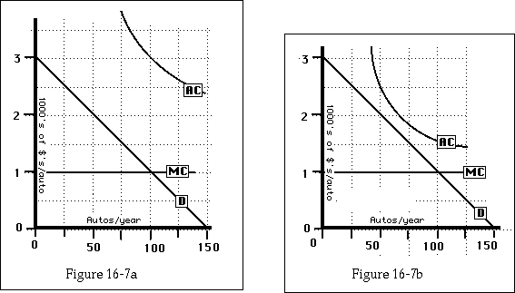
Three monopoly firms--Problems 2 and 3.
3. In each of the cases shown on Figures 16-7a through 16-7c, how large is the net loss (to consumers, producers, and government) if the firm operates as a private, profit-maximizing, single-price monopoly (or, if it cannot cover its costs, does not exist) instead of following the rule for efficient production suggested in this chapter?
By "net loss" here, I mean the number of dollars per year that, divided in some way between producers and consumers, could leave them exactly as well off with the private monopoly as they would be without the extra money but with an efficient monopoly. Note that one way of dividing $100 between me and you is to give me $200 and take $100 from you: $200 + (-$100) = $100.
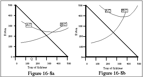
Demand and cost curves for Minnokarp fish
farm--Problem 4.
4: Figures 16-8a and 16-8b show two alternative sets of cost curves that the Minnokarp fish farm might face. Answer the following questions for each:
a. If the firm is a monopoly and cannot price discriminate, how much does it produce? What is the price?
b. If the government put the firm out of business, how much worse off would the consumers be?
c. At what price and quantity would a bureaucrat-god want the fish farm to produce?
5. Much of the United States became private property through homesteading. Whoever first claimed the land and worked it for a fixed number of years owned it. As the frontier moved west, any particular piece of land was first not worth farming (costs higher than benefits), then just worth farming, and then more than worth farming (benefits higher than costs). Under the homesteading law, at what point in this process would settlers start to farm the land? What can you say about the efficiency of this way of turning over the land to private ownership? Compare it to the alternative of auctioning off the land and using the income to reduce taxes.
6. Do you think that this book was sold to you at a price equal to the marginal cost of producing it? If not, would you be better or worse off if there were a law requiring publishers to sell books at marginal cost? Discuss.
7. We have not discussed the efficiency of monopolistic competition or oligopoly. Do you think they are efficient? Justify your answer.
Two interesting discussions of rent seeking are:
Terry Anderson and P. J. Hill, "Privatizing the Commons: An Improvement?" Southern Economic Journal, Vol. 50, No. 2 (October, 1983), pp. 438-450. (April, 1975), pp. 173-179.
Gordon Tullock, "The Welfare Costs of Tariffs, Monopolies and Theft," Western Economic Journal, Vol. 5 (June, 1967), pp. 224-232. this is, so far as I know, the first and best analysis of rent seeking.